
After doing a little bit of thinking about UI in part 1 of this article, it would be great to start producing some actual pictures of stars.
As I often do in my posts, this isn’t a tutorial that gives you the final answer (though you could skip ahead and grab the final result), but it also shows part of the process. Sometimes we’ll have to put some thoughts into it, and sometimes we might have to backtrack a little bit.
Obtaining Stars Data
If you are using Starpro, you can skip this part.
For a LatLong image to put on a sphere
Maybe the easiest way to obtain data is to download a panorama of the sky. There are multiple maps available from multiple space agencies. You can download a 6K map from the European Southern Observatory or even a 40K image generated from billions of data points in the Gaia project. NASA’s Scientific Visualization Studio also has some cool maps in both Celestial and Galactic coordinates.
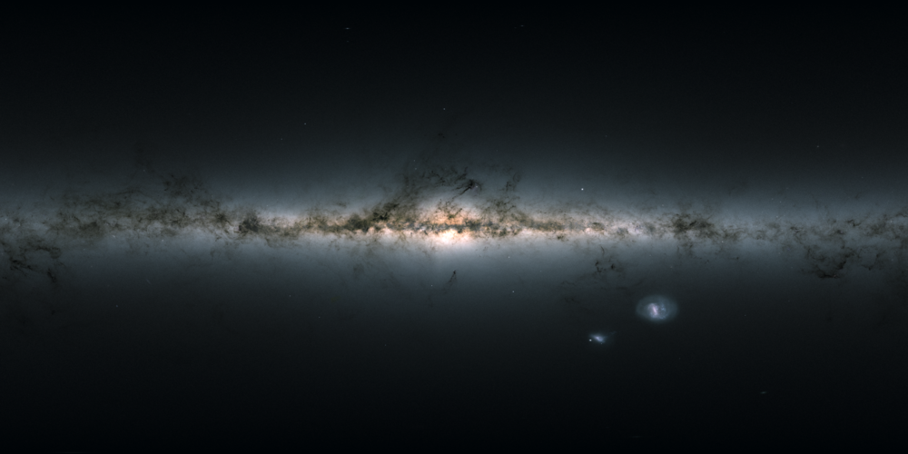
A 1K preview of the 40K map available on the Gaia project’s website (Galactic Coordinates).
To Render Points using Higx PointRender.
One of the issues that come with LatLong images is usually the UV seams, particularly at the poles. Another issue is the often limited resolution or requiring very high definition maps, which can considerably slow down Nuke. Since stars are perceived from Earth as little points in the sky, rendering a point cloud with something like Higx PointRender or a similar tool could produce good-looking results.
Unlike Starpro, PointRender doesn’t come bundled with star data, so we will need to find a way to bring our own data. As we’ve established in a previous blog post, EXR files are actually quite suited to store point cloud data, with each pixel representing a point.
There are many datasets relating to stars, known as astronomical catalogues (Wikipedia List), with a few of the most famous being Hipparcos, Tycho, and recently Gaia. The Gaia mission, in particular, is of interest to me. It is still ongoing, and the data is being released in chunks. The first part was released in September 2016, the second part in April 2018, and the Full catalogue will be released in 2022, with a beta release last month (December 2020). This is a massive catalogue with 1.8 BILLION listed objects (Gaia doesn’t map stars only). This is probably overkill for our needs, and the full dataset is a whopping 1.3TB when compressed.
Luckily, a smaller dataset is available, which we will be using as a test for this exercise: As part of Gaia’s first data release, a smaller dataset cross-referenced with Tycho was published and is only 600MB compressed. This dataset is far from perfect, however. It doesn’t contain the brighter stars in our sky, nor does it have colour information for the stars it does contain. I picked this dataset as an intro because somebody else has done most of the work for me, as you’ll see in the next paragraph.
There isn’t a very straightforward way of bringing CSV data into Nuke as pixel information, but Houdini is a perfect bridge to bring in that data. The amazing team at Entagma made the tutorial below, explaining how to bring the data into Houdini. There is also a text version of this tutorial with all the python code provided here.
You don’t need to be an expert Houdini user to follow along. There is very little you need to figure out by yourself, but a good understanding of Python will definitely help. If you don’t wish to do this whole process yourself, I’ll share the resulting EXR file a bit lower.
If using the Python script that downloads the CSV data provided by Entagma, please know that the URL of the CSV data has changed since and that you need to update line 6 of the code to read:
url_template = 'https://cdn.gea.esac.esa.int/Gaia/gdr1/tgas_source/csv/TgasSource_000-000-{:03d}.csv.gz'
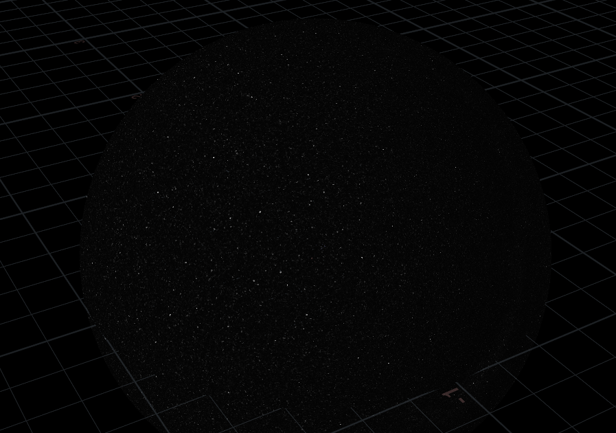
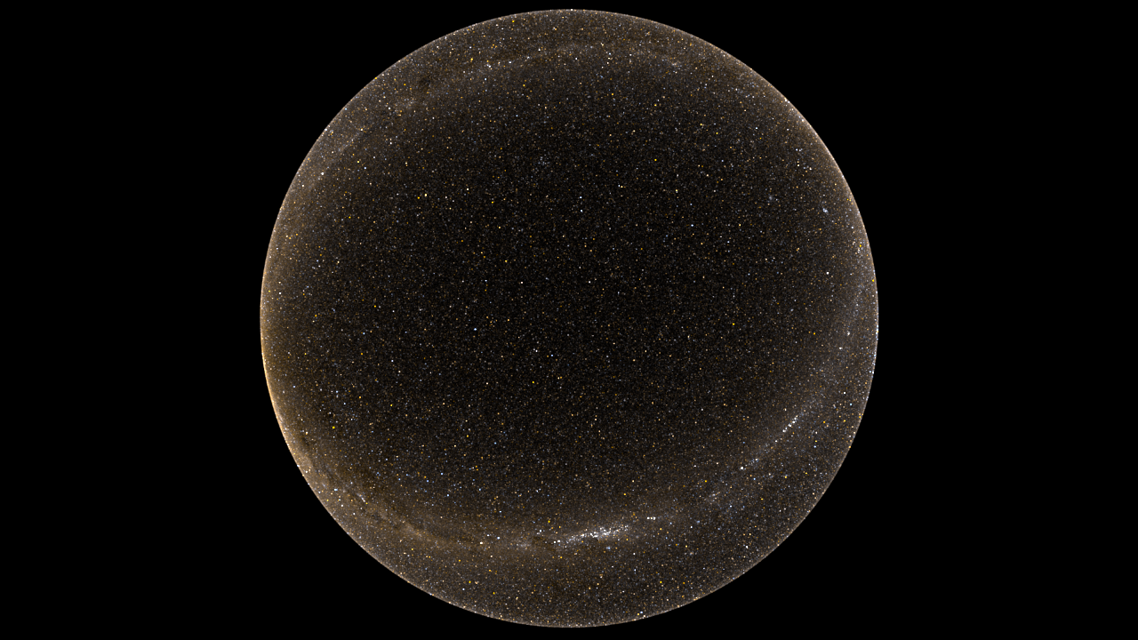
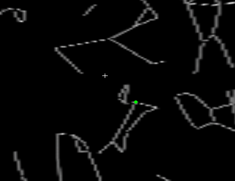
Here is the result I’m obtaining when following the tutorial above:
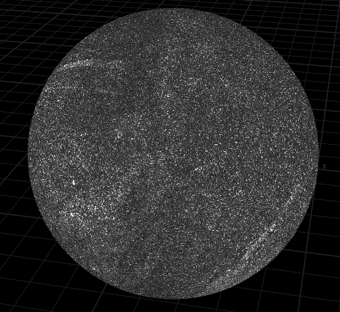
While it looks like stars, it doesn’t have the very distinctive stars or constellations we are used to observing. By looking at the CSV data and constellation data online and comparing certain star IDs, I noticed that none of the bright stars observable from the earth are part of the TGAs data dump. I could have tried to download the full dataset, but I don’t have a TB of disk space to spare or days to process the data.
After searching online for a while, I stumbled upon the open-source project Gaia Sky, a real-time universe viewer. I had a chat with the maker of Gaia Sky, Toni Sagristà Sellés, who happened to be extremely helpful, explained to me that “Gaia is not complete at the bright end at all, to the point where the sky is not recognizable if you only use Gaia stars. That is why we pre-process and crossmatch Gaia with Hipparcos so that the bright stars we all know are there“. Gaia Sky provides access to these pre-processed datasets, including a ~1GB dataset of the brightest Gaia stars, which sounds exactly like what we would want for VFX. All the data is downloadable from here: https://gaia.ari.uni-heidelberg.de/gaiasky/files/autodownload/
I chose catalog/dr2/bright and downloaded the .tar.gz file. Once I decompressed it to look at the contents, I saw a bunch of .bin files. Horrifyingly, all the files had been compiled as binary data and seemed unreadable. Luckily, with open-source software, we can dig in the code and figure out how things are done as a last resort. A quick read of the documentation (+ my conversation with Toni) gave me the information I needed, though, which is:
The meaning of each single bit in this format is described below:
- 1 single-precision integer (32-bit) – number of stars in the file
- For each star:
- 3 double-precision floats (64-bit * 3) – X, Y, Z cartesian coordinates in internal units
- 3 double-precision floats (64-bit * 3) – Vx, Vy, Vz – cartesian velocity vector in internal units per year
- 3 double-precision floats (64-bit * 3) – mualpha, mudelta, radvel – proper motion
- 4 single-precision floats (32-bit * 4) – appmag, absmag, color, size – Magnitudes, colors (encoded), and size (a derived quantity, for rendering)
- 1 single-precision integer (32-bit) – HIP number (if any, otherwise negative)
- 3 single-precision integer (32-bit * 3) – Tycho identifiers
- 1 double-precision integer (64-bit) – Gaia SourceID
- 1 single-precision integer (32-bit) – namelen -> Length of name
- namelen * char (16-bit * namelen) – Characters of the star name.
Python allows us to read binary files, so we can write our own reader based on the info above.
For that, we use the struct python module and open the file in binary mode. We then decode our bytes group by group to get all the info we need. This is a bit more complicated than a CSV, but that saves me from buying a new hard drive to download and process larger datasets.
The code below is based on the Entagma python script, with the Houdini-specific parts removed (so that I could run my tests outside Houdini, where I’m more comfortable).
import os
import struct

def read_row(fp):
    # the fp.read() method takes bytes instead of bits as an argument, so we need to divide by 8.
    # 3 double-precision floats (64-bit * 3) – X, Y, Z cartesian coordinates in internal units
    # 64 bits = 8 bytes, 8 bytes * 3 = 24 bytes
    # the first argument passed to struct unpack tells it how to interpret the binary data.
    # Here, I tell it to read the bytes left to right (big endian) with the '>' symbol,
    # and that it will contain 3 "doubles" ('ddd') which are 64-bit floats.
    x, y, z = struct.unpack('>ddd', fp.read(24))
    # 3 double-precision floats (64-bit * 3) – Vx, Vy, Vz - cartesian velocity vector in internal units per year
    Vx, Vy, Vz = struct.unpack('>ddd', fp.read(24))
    # 3 double-precision floats (64-bit * 3) – mualpha, mudelta, radvel - proper motion
    mualpha, mudelta, radvel = struct.unpack('>ddd', fp.read(24))
    # 4 single-precision floats (32-bit * 4) – appmag, absmag, color, size - Magnitudes, colors (encoded), and size (a derived quantity, for rendering)
    # Here we have 4 times 32, so 16 bytes, and we change the struct argument to '>ffff' to reflect.
    appmag, absmag, color, size = struct.unpack('>ffff', fp.read(16))
    # 1 single-precision integer (32-bit) – HIP number (if any, otherwise negative)
    # 3 single-precision integer (32-bit * 3) – Tycho identifiers
    # I combined these 4 in a single line, and changed the pattern to use 'i' for integers.
    hip, tycho1, tycho2, tycho3 = struct.unpack('>iiii', fp.read(16))
    # 1 double-precision integer (64-bit) – Gaia SourceID
    gaia_id = struct.unpack('>q', fp.read(8))[0]
    # 1 single-precision integer (32-bit) – namelen -> Length of name
    name_length = struct.unpack('>i', fp.read(4))[0]
    # namelen * char (16-bit * namelen) – Characters of the star name.
    if name_length > 0:
        # This is a bit weird, but basically each character is encoded separately in utf-16
        name = ''
        for _char in range(name_length):
            name += fp.read(2).decode('utf-16-be')

def read_bin(fp, maxrows):
    number_of_stars = struct.unpack('>l', fp.read(4))[0]
    count = 0
    while count < number_of_stars:
        if count >= maxrows:
            break
        read_row(fp)
        count += 1
    return count

def main():
    # These 2 will be replaced later with the Houdini knobs
    maxrows = 20
    directory = 'C:\Users\erwan\Downloads\gaia\catalog\dr2-bright\particles'

    files = []
    for name in os.listdir(directory):
        if name.endswith('.bin'):
            files.append(os.path.join(directory, name))
    files.sort()

    count = 0
    for fi, filename in enumerate(files):
        if count >= maxrows:
            break
        with open(filename, 'rb') as fp:
            count += read_bin(fp, maxrows - count)

# Put this at the very end of your node's code.
main()
Feel free to put print statements in there to see all the available parameters and verify it works.
Let’s put back the Houdini-specific code and simplify the code a bit. There are many parameters in the .bin files that I’m not interested in. I can “skip” decoding these chunks of bytes to save some time and reduce the amount of code (not that it would make a huge difference).
I ended up with this code:
import hou
import os
import struct
import numpy

node = hou.pwd()
geo = node.geometry()

COLUMNS = 'appmag,absmag,color,size'.split(',')
for col in COLUMNS:
  geo.addAttrib(hou.attribType.Point, col, 0.0)


def read_star(fp):
    pos = struct.unpack('>ddd', fp.read(24))
    pos = numpy.array(pos)/numpy.linalg.norm(pos)  # Because Python has 64bit precision while Houdini only 32 by default, I normalize the pos here. Also I don't care about the actual position, though some of you reading this might.
    # read bytes without even storing them to a variable just "skips" a chunk.
    fp.read(48)
    # 4 single-precision floats (32-bit * 4) – appmag, absmag, color, size - Magnitudes, colors (encoded), and size (a derived quantity, for rendering)
    appmag, absmag, color, size = struct.unpack('>ffff', fp.read(16))
    fp.read(24)
    # 1 single-precision integer (32-bit) – namelen -> Length of name
    name_length = struct.unpack('>i', fp.read(4))[0]
    # namelen * char (16-bit * namelen) – Characters of the star name.
    if name_length > 0:
        fp.read(name_length*2)

    # Create the Houdini points
    point = geo.createPoint()
    point.setPosition(hou.Vector3(*pos))
    point.setAttribValue('appmag', appmag)
    point.setAttribValue('color', color)
    point.setAttribValue('size', size)

def read_bin(fp, maxrows):
    number_of_stars = struct.unpack('>l', fp.read(4))[0]
    count = 0
    while count < number_of_stars:
        if count >= maxrows:
            break
        read_star(fp)
        count += 1
    return count

def main():
    maxrows = node.parm('maxrows').eval()
    directory = node.parm('directory').eval()

    files = []
    for name in os.listdir(directory):
        if name.endswith('.bin'):
            files.append(os.path.join(directory, name))
    files.sort()

    count = 0
    with hou.InterruptableOperation('Reading BIN', 'Reading Files', True) as op:
        for fi, filename in enumerate(files):
            op.updateLongProgress(fi / float(len(files)-1), os.path.basename(filename))
            if count >= maxrows:
                break
            with open(filename, 'rb') as fp:
                count += read_bin(fp, maxrows - count)

# Put this at the very end of your node's code.
main()
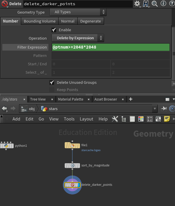
With 7.7Million points, this one is a rather dense point cloud.
I don’t think I need 7 Million points, but I think a 2k map (2048*2048) would be a reasonable size to handle in PointRender, so the first thing I do in Houdini is sorting the stars from brightest to dimmest, then only keep the ~4M brightest stars:
Next, I want to convert the magnitude to a value that we’re more used to in VFX, where the highest number is brighter and the lowest darker. This was covered in the Entagma tutorial, but for reference, here is the VEX code I’m using for that. For now, I will store it as colour (Cd) so that I can preview it in the viewport.
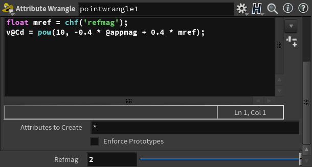
I found that a Reference magnitude of 2 gives me a relatively “naked eye” look for the stars.
The next thing I’d like to do is assign a colour to the stars. Right now, they are all a shade of grey, based purely on their brightness, but the Gaia Sky data included a value for the colour. However, that value is a float, and that isn’t how we are used to representing colours in VFX. Again, looking at the documentation, I can see that “The RGB colour of stars uses 8 bits per channel in RGBA, and is encoded into a single float using the libgdx Color class“. Oh, so this is more packing data into bits. Since I don’t know how to do that in VEX, and I’m not getting results after a short googling section, let’s go back and handle it in Python. The docs tell me it’s 4*8bit ints, put together in order ABGR.
Our Python code becomes:
import hou
import os
import struct
import numpy

node = hou.pwd()
geo = node.geometry()

COLUMNS = 'appmag,size'.split(',')
for col in COLUMNS:
    geo.addAttrib(hou.attribType.Point, col, 0.0)
geo.addAttrib(hou.attribType.Point, 'Cd', hou.Vector3())


def read_star(fp):
    pos = struct.unpack('>ddd', fp.read(24))
    pos = numpy.array(pos)/numpy.linalg.norm(pos)  # Because Python has 64bit precision while Houdini only 32 by default, I normalize the pos here. Also I don't care about the actual position, though some of you reading this might.
    # read bytes without even storing them to a variable just "skips" a chunk.
    fp.read(48)
    # 4 single-precision floats (32-bit * 4) – appmag, absmag, color, size - Magnitudes, colors (encoded), and size (a derived quantity, for rendering)
    appmag, absmag, a, b, g, r, size = struct.unpack('>ffBBBBf', fp.read(16))
    fp.read(24)
    # 1 single-precision integer (32-bit) – namelen -> Length of name
    name_length = struct.unpack('>i', fp.read(4))[0]
    # namelen * char (16-bit * namelen) – Characters of the star name.
    if name_length > 0:
        fp.read(name_length*2)

    # Create the Houdini points
    point = geo.createPoint()
    point.setPosition(hou.Vector3(*pos))
    point.setAttribValue('appmag', appmag)
    point.setAttribValue('Cd', hou.Vector3(*[r, g, b])/255.0)
    point.setAttribValue('size', size)

def read_bin(fp, maxrows):
    number_of_stars = struct.unpack('>l', fp.read(4))[0]
    count = 0
    while count < number_of_stars:
        if count >= maxrows:
            break
        read_star(fp)
        count += 1
    return count

def main():
    maxrows = node.parm('maxrows').eval()
    directory = node.parm('directory').eval()

    files = []
    for name in os.listdir(directory):
        if name.endswith('.bin'):
            files.append(os.path.join(directory, name))
    files.sort()

    count = 0
    with hou.InterruptableOperation('Reading BIN', 'Reading Files', True) as op:
        for fi, filename in enumerate(files):
            op.updateLongProgress(fi / float(len(files)-1), os.path.basename(filename))
            if count >= maxrows:
                break
            with open(filename, 'rb') as fp:
                count += read_bin(fp, maxrows - count)

# Put this at the very end of your node's code.
main()
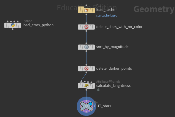
We now have an RGB value as we’re used to. I can re-load all my stars, cache the Houdini geo, and modify my VEX (Point Wrangle) from before so that the magnitude multiplies the colour intensity instead of replacing it. After running the code, I noticed there’s a fair number of points with no colour information. These are all fairly dark stars, so to simplify my life, I remove these.
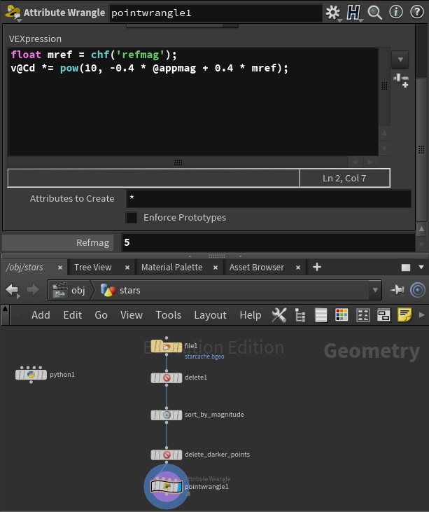
I then do a bit of housekeeping, naming nodes, and adding a Null as my output.
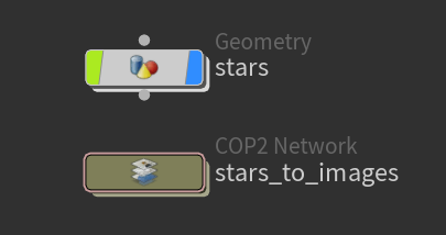
Time to export these to Nuke. For this, we will use Houdini’s COP (compositing) tools. Back in the object context, add a COP2 node.
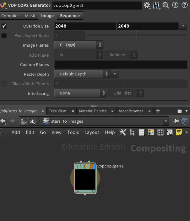
Inside the COP2 Network, add a VOP generator and set the resolution to be 2048*2048, and just RGB (I don’t care about alpha right now):
Now, within the VOPCOP, we wire the nodes as follows:
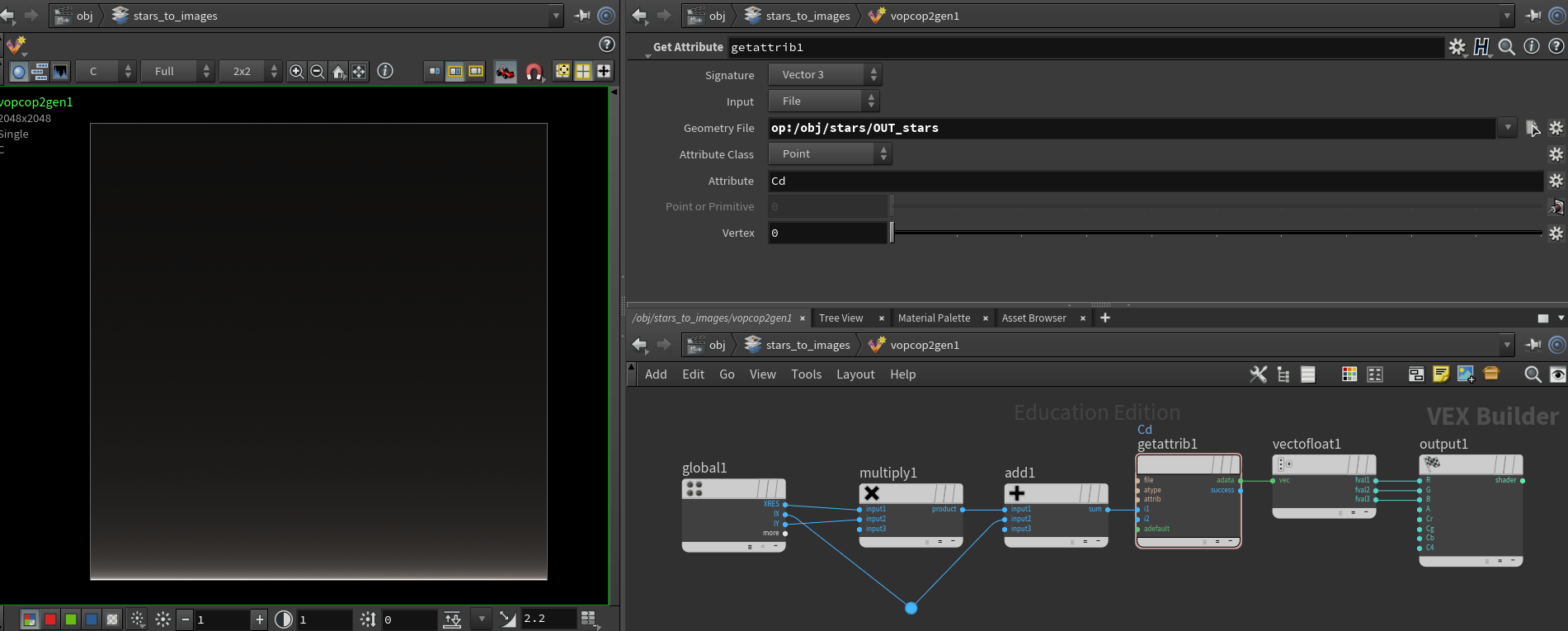
The flow is:
On the left, the global node provides us with a bunch of variables. I’m interested in XRES (Resolution in X), IX (integer value of current pixel X position), IY (int value of pixel Y position). If I multiply the Y position by the X resolution, then add the X position, each pixel now has a single value, with the bottom left corner having the value 0, the one to the right of it a value of 1, then 2, then 3, etc… When it reaches the end of the first line, it will go back to the left, and start with the value 2048, then 2049, 2050, etc…
From this int value, using the getattrib node, set up as per the screenshot above, we obtain the Cd attribute, which is a vector. Finally, with vectofloat, we convert the vector to 3 floats and assign them to R, G, B in the output.
Since we had sorted our stars by brightness, the final result is a sort of noisy vertical gradient, which makes a lot of sense since we write the values line by line.
We now need to get the stars’ positions. We can copy our VOPCOP node, as it’s the exact same VOP graph but with the P attribute instead of Cd.

We can now write these out as EXRs:
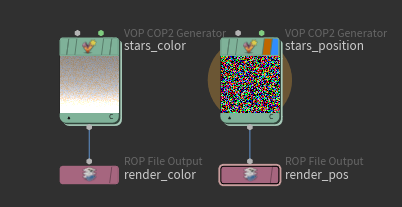
We’re now done with Houdini!
In Nuke, we can now bring in these 2 images and format them in a way that PointRender likes:
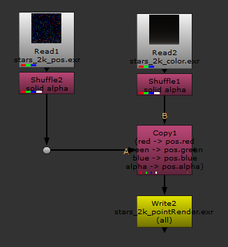
We could have done it in Houdini, but I’m a lot more familiar with Nuke, so I decided to assemble it there.
We can then plug in PointRender, a camera, and a saturation node because I wanted to check that the colors actually came through, and get this result:
If we need to render fewer stars and only keep the brightest stars to speed up the render a bit, all that is needed is cropping the top of the 2K map since all the brightest stars are at the bottom.
Orientating the stars to get an accurate sky from the current location and date
If you are using StarPro or my EXR file above, the stars should be nearly in the same location when rendered with the same Camera. I had to rotate my stars 90 degrees to make them line up with Starpro. It can be done in Houdini with a Transform before exporting the pos pass, though I did it in Nuke directly using my VectorRotate Node. StarPro will also adjust the star’s size, which we have not exported from Houdini, as by default, PointRender doesn’t really accept a point Size map. One thing I might experiment with in the future is to encode the size in the position pass as the vector magnitude, which might let us achieve a size via a defocus or another type of convolution.
If you are using a LatLong image, you may notice that the base orientation is different.
For a map in Celestial Coordinates, you will need to mirror the map horizontally and rotate the sphere by -90 in Y.
You will need to mirror the map horizontally for a map in Galactic Coordinates and rotate the sphere by roughly -28.9, 176, -58.8 in XYZ, with ZXY rotation order.
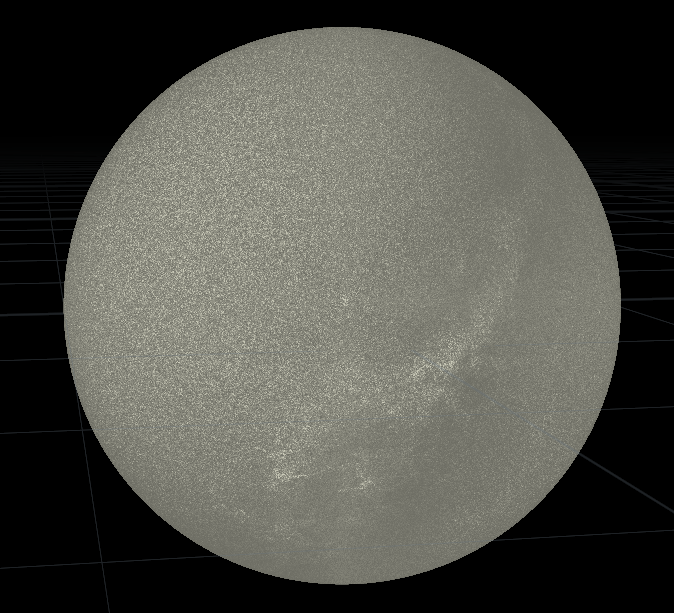
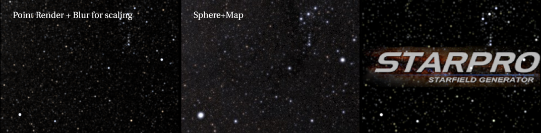
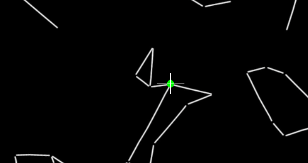
We now have multiple methods of rendering stars that should all pretty much line up:
However, in Part 1 of this article, I said my goal was to be able to pick my location on earth, the time and date, and have the sky show the correct stars.
For simplicity, and because we didn’t store that data, we’ll ignore the fact that stars are all moving in different directions very slowly (well, very fast, but slow from our point of view) and stick to the idea of the celestial sphere, where nearly all motion is due to the earth’s rotation.
Usually, when we make cameras for VFX, we don’t think of the absolute orientation based on the celestial circle but in terms of the ground. We set the ZX plane parallel to the floor (at least in Nuke, some other software use XY as the floor). We also don’t always really care where is North, South, East, or West. In our case, we will need to care about orientation. The first thing to do was deciding which axis to map to the north. I decided that north would be towards -Z for 2 reasons: It’s the direction a default Nuke Cam points to, and if I put a picture of a compass on a horizontal card, that’s how it will map by default.
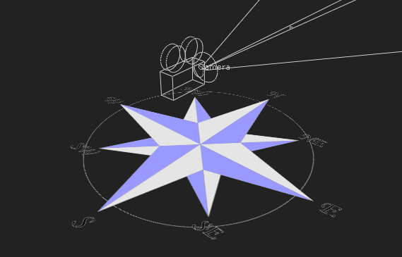
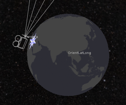
Now, all we need to do is that when we pick a Latitude and Longitude with the widget we created in part 1, the whole scene needs to “stick” to the surface of the earth.
Above is an illustration of what this would look like if there were an actual planet there, but in this case, we don’t need that planet to be present; all we need is the rotation values.
To achieve that, I connect an axis above the Camera, which I expression link to our NoOp with the world map:
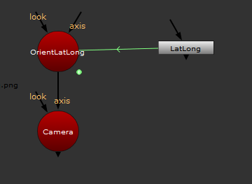
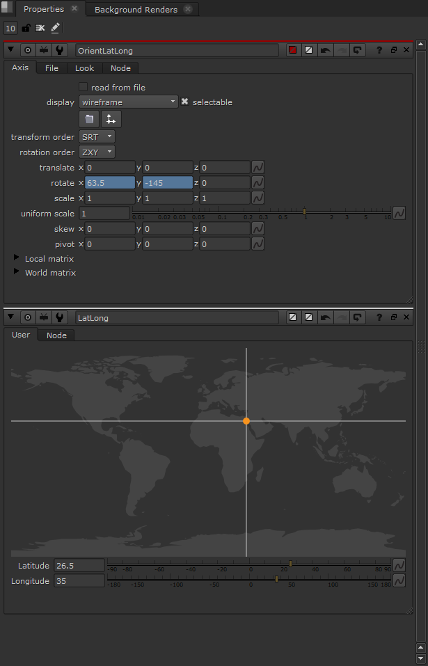
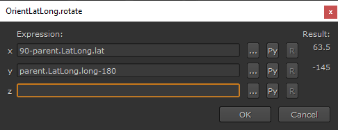
This orients our scene properly (assuming your North was -Z) for the geographic location at an undetermined point in time.
Since it’s quite likely that the scene was NOT properly aligned with -Z matching North, I decided to add a “Compass” rotation knob, which will allow me to rotate the North’s position.
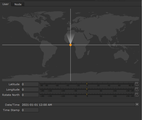
I also think it would be nice to have a visual representation on the world map of our current orientation:
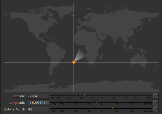
This requires going back to the code we wrote in part 1 and modify it slightly to draw a little preview of our Field of View. I’m not going to detail how I drew this, but the quick version is that I calculate the orientation of our camera, then in the paintEvent of the custom widget, I draw a polygon filled with a ramp in the proper position. I think I will also later consider the field of view of the camera so that the triangle I draw has the proper angles. I will post the final code to download at the bottom of this article, so you will be able to see all the details there.
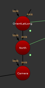
Back to our 3D scene, the Rotate North value goes in the Rotate Y of an axis connected this way:
Our camera is now, in theory, oriented the right way. However, it is still oriented at an arbitrary time and date. You might remember that I rotated the stars in our dataset earlier by 90 degrees to match StarPro. That might affect our coordinates as well. Let’s do a bit of reading to figure out what the celestial coordinates are based on. This article tells us:
The rather arbitrary choice made by astronomers long ago was to pick the point at which the Sun appears to cross the celestial equator from South to North as it moves through the sky during the course of a year. We call that point the “vernal equinox”.
That falls on March 20 most years, but possibly at different times of the day. Alright, that doesn’t help me that much, but it was nice of astronomers to define their coordinate system relative to my birthday. Since I don’t need to be extremely precise, I could line up the stars at one arbitrary point in time, let’s say January 1st, 2021, at midnight UTC. Then for any other date and time, I can rotate the earth by the right amount. Google tells me that the earth rotates by 360 degrees in 23h, 56min, and 4sec.
I can pick an arbitrary star, make sure it’s lined up properly, and then verify with a second star to make sure my coordinate system isn’t flipped or anything.
First, let’s add a final Axis: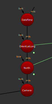
Let’s leave this axis alone for now. We’ll use it to find the right time very soon.
Now, let’s look at Sirius, the brightest star. From London (easier since London is in UTC, don’t need to do time zone conversions) on 01/01/2021 at midnight, Sirius should be at an altitude of 21.82 degrees and 179.44 degrees towards the south (I just googled the coordinates, and trusting that the results are from people who actually know what they are doing, unlike myself). By googling Sirius’s RA and DEC, and applying some math, let’s bring in just Sirius in nuke:
from math import radians, cos, sin

sirius = nuke.createNode("Sphere")
sirius.setName('Sirius')
sirius['uniform_scale'].setValue(0.05)

ra = 6*(15) + 45*(1.0/4) + 8.92 * (1.0/240)  # 6h45min8.92sec
ra *= -1  # Mirror Longitude (like we had to mirror textures)
dec =  -(16 + 42*(1.0/60) + 58.017 * (1.0/3600)) # −16° 42′ 58.0171″
lon = radians(ra)
lat = radians(dec)

# Transform spherical coordinates to coordinates on the unit-sphere.
x = cos(lat) * cos(lon)
y = sin(lat)
z = cos(lat) * sin(lon)

sirius['translate'].setValue((x, y, z))
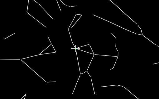
For the math, I have explained how to calculate a 3d coordinate on a sphere from a latlong map in some of my previous tutorials. We plug in the coordinates of Sirius and verify that it falls in the right place.
Using a map of the constellations is convenient to check the location.
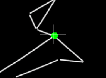
Then, on our map, pick London’s location and rotate the camera so that it’s pointing at the coordinates above (altitude of 21.82 degrees and 179.44 degrees towards the south).
By rotating the Y-axis of our new Axis “DateTime”, we should have Sirius right at the center of the frame. I found that a value of 10.6 lines it up nearly perfectly:
Now let’s confirm that this wasn’t pure luck and repeat the operation with a second star.
Let’s see if Betelgeuse will fall in the right place.
from math import radians, cos, sin

betelgeuse = nuke.createNode("Sphere")
betelgeuse.setName('betelgeuse')
betelgeuse['uniform_scale'].setValue(0.05)

ra = 5*(15) + 55*(1.0/4) + 10.30536 * (1.0/240)  # 05h 55m 10.30536s
ra *= -1  # Mirror Longitude (like we had to mirror textures)
dec =  7 + 24*(1.0/60) + 25.4304 * (1.0/3600) # +07° 24′ 25.4304″
lon = radians(ra)
lat = radians(dec)

# Transform spherical coordinates to coordinates on the unit-sphere.
x = cos(lat) * cos(lon)
z = cos(lat) * sin(lon)
y = sin(lat)

betelgeuse['translate'].setValue((x, y, z))
Google tells me it should be at 44.83 degrees of altitude, 196.8 (South, South-West).
It looks like we’re all good; our camera is now oriented as it would have been on January 1st, 2021, at midnight.
Using the same techniques we used in Part 1, I will now add a dateTime widget to the custom widget. For storage, I will use an int knob, which will store the date/time as the number of seconds since January 1st, 1970 (This is standard in computer science, and how dates and times are often stored). Because I’m using an int as storage, we won’t be able to calculate the rotation for less than a second, but it’s so small that I don’t think it will be an issue. I will keep this knob visible, even though it might look a bit odd, for convenience so that keyframes can be added or deleted. I could also implement these features in my custom knob, but sometimes I prefer to let Nuke handle things its own way.
I then need to connect the Date/Time knob to the Time Stamp knob.
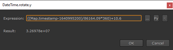
Once this is done, I expression link our DateTime Axis Y rotation to the time stamp.
I know that I lined up my stars in 2021/01/01 00:00, which is a timestamp of 1640995200, and had a rotation value of 10.6.
I also know that it takes 86164.09 seconds for the earth to rotate 360 degrees. (Later Edit: That’s actually the timestamp for 2022, so I changed it later)
Let’s do a final check and find Sirius at a different date. Google tells me that on February 7th, 2001, at 12:51 am (10 years ago from the time I’m writing this line), Sirius was at altitude 10.03 and direction 226.41.
We’re slightly off-center but pretty close.
Packaging this into a gizmo or group
Now that everything works as expected, it would be great to clean it up and make it convenient to use again and again in the future. I would like to have a group with a single input for a camera, which would output a camera pointed at the right part of the cosmos.
We can start by creating an empty group, and adding all the knobs we had on our NoOp on that group first.
Then, we move our nodes within the group.
One challenge we will be facing is that we currently have a few Axes above our camera:
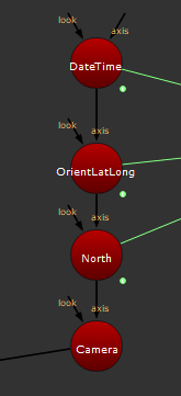
To maintain the same result within a group will require a bit of re-wiring. Any time I make a gizmo that deals with Cameras, I like to use DummyCam as a way to reliably access the cam within the group.
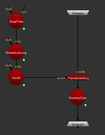
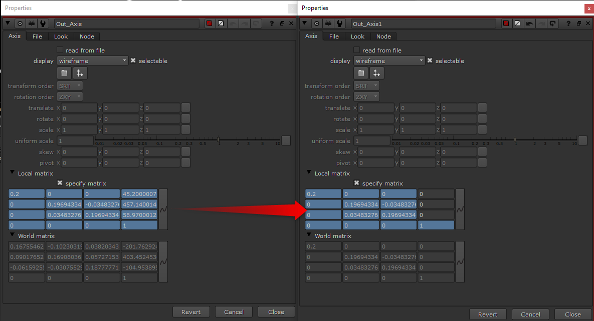
I also use the TransformAxis node which allows me to obtain the same result as above but within a group (the node allows does the same operation as connecting an axis above another, but from ‘under’, similar to a transform geo). Hopefully, this screenshot makes more sense:
To make the camera behave like our stars are infinity large (while in reality, they are on a little sphere), we need to ensure that the camera’s position is always at 0, 0, 0. Looking at the world Matrix of our DummyCam we can see if the camera is at the origin:
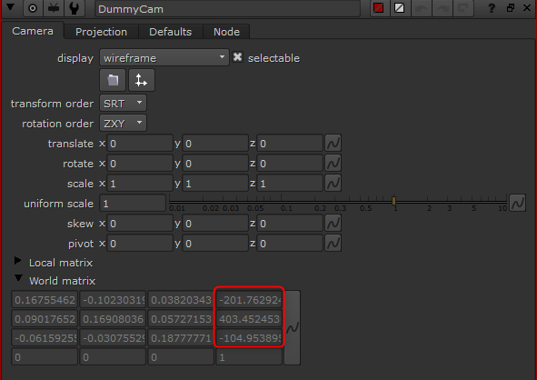
The values should be 0, 0, 0
We could add another Axis, and expression-link the translation values to the parent world matrix. However, in this case, I know that the only place these translation values can come from is the input, and I also know that the TransformAxis node applies these values to my world matrix. I can go into the TransformAxis node and remove the expression for these few values:
The camera will now always be at the origin, and nothing other than the rotation will affect it (scale and skew could, but not often used on cameras).
Final Test
Finally, to make sure the tool gives plausible results, I decided to try to reproduce a picture I took a few weeks ago on a trip. I knew the lens and sensor size, as well as the time I took the picture and the rough location. However, I didn’t write down the orientation of the camera, so these would need to be matched by eye.
The image is also a long exposure, so I would need to animate the time and enable motion blur out of PointRender.
This showed that the expression I was using for setting the time was lacking precision, as the rotation values were huge. This made me add a knob “reference timestamp”. Instead of rotating the earth around the right number of times since 1970, I use the reference number to ensure the rotation at that date is less than 360 degrees, giving me a lot more precision to achieve smooth star trails. I might revisit this in the future, but for now, it does the job.
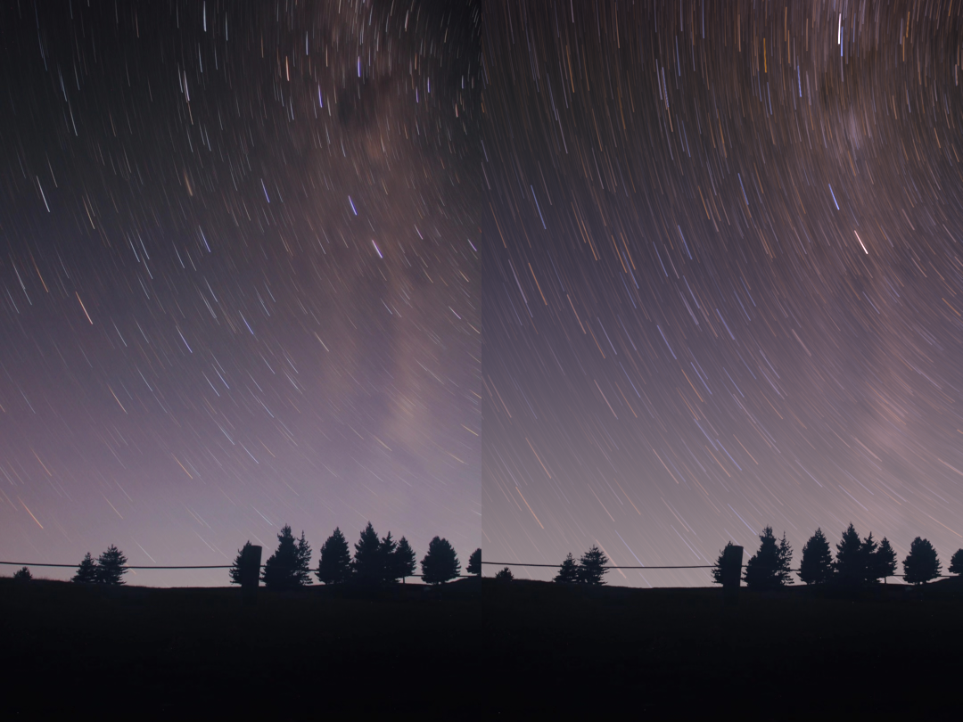
The whole sky on the picture on the right is generated in nuke. The sky itself is a ramp, and the stars (including the milky way) are coming from PointRender. I ignored lens distortion and eyeballed the camera orientation, but overall it’s in the right ballpark. It’s interesting to me that some stars seem to be blue on the reference image but orange on the generated sky, and vice versa. It also seems like the brightness values aren’t entirely accurate as I had to color correct the image to approach the balance from the reference. The exposure is probably a bit too long as well.
Get the nuke and python scripts on Gist: Celestial Camera
I learned a lot while writing this post and I hope some people will learn a trick or two from reading it. This was not a linear journey, and I hit a few bumps on the road, but I’m glad that I managed to get something working in the end. Don’t hesitate to ask questions.
absolutely amazing stuff
Thank you
This is great man!
really amazing stuff, well done,
I was wondering…
I’m having an QT module error. AM I doing somehing wong?
Thanks
M
You’re not necessarily doing anything wrong. Which version of nuke are you using? PySide2 was introduced with Nuke 11 if my memory is correct so anything older will probably complain about the module missing.
If it’s a different error, feel free to email me the error message and I’ll take a look.
This is great, thanks for walking through it! I was banging my head on the Gaia data not finding the milky way so this was a huge help! I did notice a few issues with the Python code. The way it’s currently formatted on here, it’s not designed to process all the data with maxrows set to 0 the way it was built in the Entagma tutorial because the main function breaks on count being more than or equal to maxrows, so if maxrows is 0, it will break immediately, turning maxrows into only functioning for the exact number of rows desired. It’s nice for 0 to be a full load like in the previous tutorial. Also, the read_star() function the way it’s currently set up only processes the first line, so you only get the number of stars per bin file, instead of looping through the lines. I adapted the code for both and would be happy to share the update if it’s helpful for anyone. Regardless, thanks so much, super useful stuff!
Hi, thank you for the heads up about the broken while loop exit condition, all my special characters got replaced on a previous edit, and looks like I have sometimes put > instead of < when I was fixing it. Regarding the read all on 0, somehow it's in the video version of the entagma tutorial but not the written version that I based the code on, so I didn't even think about it. All that's necessary is changing line 40 from
if count >= maxrows:toif maxrows and count >= maxrows:A master class of Houdini, thanks a bunch!