Last week we started playing with Higx PointRender, and we saw how it wasn’t really a particle system as we’re used to. Let’s dive a little deeper to understand what differs between this method and Nuke’s particle system, see how we can get our points to behave more like particles, and what are the limitations we’re going to run into.
What is a particle system?
Summarized from Wikipedia:
A particle system is a technique in game physics, motion graphics, and computer graphics that uses a large number of very small sprites, 3D models, or other graphic objects to simulate certain kinds of “fuzzy” phenomena, which are otherwise very hard to reproduce with conventional rendering techniques.
Typically a particle system’s position and motion in 3D space are controlled by what is referred to as an emitter. The emitter acts as the source of the particles, and its location in 3D space determines where they are generated and where they move to. The emitter has attached to it a set of particle behavior parameters. These parameters can include the spawning rate (how many particles are generated per unit of time), the particles’ initial velocity vector (the direction they are emitted upon creation), particle lifetime (the length of time each individual particle exists before disappearing), particle color, and many more.
During the simulation stage, the number of new particles that must be created is calculated based on spawning rates and the interval between updates, and each of them is spawned in a specific position in 3D space based on the emitter’s position and the spawning area specified. Each of the particle’s parameters (i.e. velocity, color, etc.) is initialized according to the emitter’s parameters. At each update, all existing particles are checked to see if they have exceeded their lifetime, in which case they are removed from the simulation. Otherwise, the particles’ position and other characteristics are advanced based on a physical simulation, which can be as simple as translating their current position, or as complicated as performing physically accurate trajectory calculations which take into account external forces (gravity, friction, wind, etc.). It is common to perform collision detection between particles and specified 3D objects in the scene to make the particles bounce off of or otherwise interact with obstacles in the environment.
After the update is complete, each particle is rendered.
As you can see from reading the description, what we did last week isn’t quite fitting with the general method. While we did use it to render a large number of small graphic objects to simulate a “fuzzy” phenomena, we sort of skipped the whole emission/simulation phase to go straight to the rendering.
The differences between using Position Data and Nuke’s particle system
Nuke’s particle system fits the Wikipedia description much better than the techniques we’ve played with with PointRender. In a sense, that might be one of the strengths of PointRender. It doesn’t need to to go through these expensive steps of emission and simulation.
If we break down how a nuke particle is generated/rendered (assuming no substeps) the following happens on each frame:
- Check if the emitter should emit particles
- Add new particles (with their properties/channels) to the existing particles.
- Current properties of each particle is either based on the previous frame, or the initial properties as given by the emitter. We need to calculate the new properties:
- Resolve forces
- Resolve collisions
- Update lifetime
- Check other properties that are based on lifetime or other, such as ParticleCurve or ParticleExpression
There is a total of at least 11 properties to update (there might be more that I’m not aware of). They are: age, color, position, opacity, size, mass, acceleration, velocity, frame, force, channel).
- Render Particles, which might include replacing each particle with a sprite or geometry.
Let’s compare that with the techniques we have done last week:
- Use nodes to define two properties: color and position
- Render Particles, as a dot.
There is visibly less calculations involved. Step 1 of rendering with PointRender can be processing intensive based on the nodes used to generate the color and position, but there is much less properties to take into account (2 vs 11+). Some other particle systems, like in Maya or Houdini can keep track of even more properties per particle, such as Rotation, Temperature, or any arbitrary attribute the artists need to achieve the required look.
Another big difference we notice, is that with a simulated particle system, to calculate a frame, you need to know the state of the particles in the preceding frame. To calculate the state of the preceding frame, you need to know about the frame before it, etc.. That means a particle system will need to calculate every frame before the current frame in order to calculate the current frame. This is why there is usually a knob to control the first frame of the simulation, otherwise we would be in an infinite loop there. With PointRender we don’t need to know about any other frame, we just render the current one.
All of that sounds like PointRender only has the advantage on traditional particles, but that is not the case, there are a few things that Particles can handle that PointRender cannot handle right out of the box.
In most cases, point render will work with a fixed number of points, based on your image resolution. You could try having a resolution that changes from frame to frame, but in most use cases you’ll work with a fixed resolution. That means if you go for a million points, PointRender will have to evaluate a million points, all the time. With an emitter the number of particles is fluid, and you can start with just a few particles and increase the number as needed, or even have particles spawn new particles on specific conditions. You could implement an emitter type of node for PointRender but it wouldn’t be super straightforward.
You can’t do physics simulation (wind, gravity, collisions, etc..) with the PointRender workflow, as you do not have access to the state at the previous frame, and while you could with a time offset, it might not be a fully resolved state.
Finally, you can only render points, not any other type of particles (geo or sprite).
Each method has advantages and inconveniences, but with our experiments today, we’ll introduce some of the good stuff from Particles to PointRender, and while we’re at it, we’ll introduce some of the bad as well.
Simulating our points
As mentioned earlier, in order to simulate a progression of the position of our points, we need to have access to the points positions at the previous frame, and use that as our starting point. That is not really hard to achieve, but a bit convoluted in Nuke. We need to setup what we call a feedback loop.
There are two good articles talking about setting up feedback loops in nuke: The SetLoop tool from Max Van Leeuwen, Sprut and the article about the blink exploit by Mads. You can read these if you want to dive deeper into feedback loops, but the basic idea is very simple: Render the image to disk, and reload it as the base for the next frame.
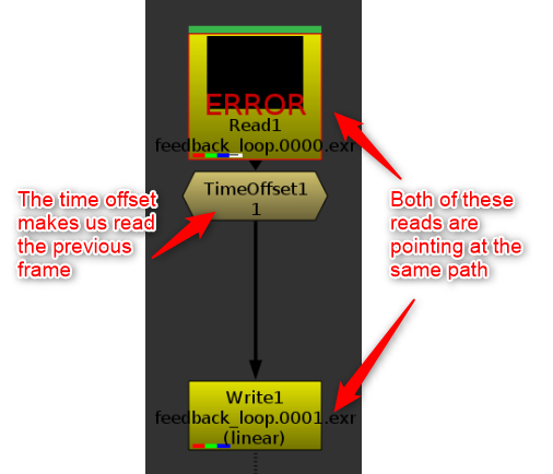
The most basic feedback loop.
The problem with the loop above, is that since nothing was ever rendered, it will error forever. You also have to be aware of the frame range set on the Read node, because once we start rendering, we don’t want the read node to ignore our new frames. What I like to do is setup my initial seed with an expression driven switch to decide what to read. See this basic example:
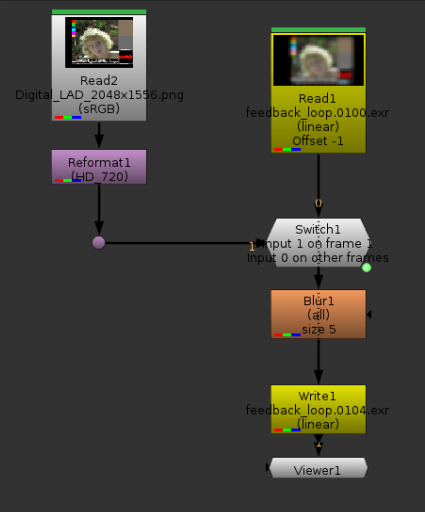
I this feedback loop, I use Marcie as my original seed, and then on each frame blur her by 5 pixels. The blurred image is read in the next frame, then blurred again, etc.. Note the blur is not animated. Somehow Nuke was refusing to render with the TimeOffset node, so I set the offset in the read node directly.
Marcie, getting blurrier and blurrier.
I will admit, not particularly impressive so far. The good news however is that in terms of setup, we’re pretty much done. Let’s take this idea into a point cloud world now. For the same reason as last week, I will not be using any Higx node so that I can share the code freely here. I’m going to replace Marcie with a Volumetric Cube generator I made for the occasion. What I hadn’t noticed until I was done with it is that my Volumetric Cube generator is pretty much a CMS Pattern, except each value is only in 1 pixel, and I don’t need to necessarily have the same number of samples in x, y and z.
In the loop, I will replace the blur with a grade, in which I will add an offset in green (basically moving the cube down slightly, as we remember green represents our Y position).
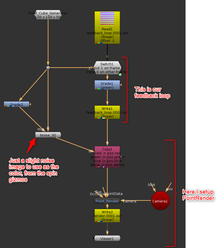
The setup with the cube generator which falls due to being moved in Y slightly on each frame.
The result of the PointRender, with the position map inserted in the lower left corner.
This is our first “simulated” point cloud. We can’t really talk about physics at that point, this is not even a simplified gravity.
Forces and velocity
We could already call the Grade node above a force. On each frame, it applied a downward force on the points.
A force is really a 3D vector that needs to be applied to the points. In order to apply more forces, we can keep doing that. Gravity: -0.2 in y, Wind: +0.3 in x, etc..
We could keep going this way and have multiple nodes each moving the points one after the other. This is what the default nodes in the Higx suite do in a way, without the feedback loop.
Another way we could approach this would be to add a velocity layer, and have each force applied as a vector on the velocity channels. Vector additions are quite simple mathematically, and look like this:
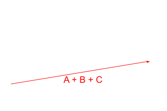
Addition of Vectors A, B and C. Each of the vectors could be a force, and the red vector our Velocity channel.
In such a setup, we would add all the forces, and only once all the forces have been calculated we would move the point.
Doing it this way does not make a visible difference with a setup like we had above, but it does make one difference, which is that this way, all the forces are applied at once instead of one after the other.
Imagine the situation where we have a predefined area that is the only area receiving a force (a circle).

If only the points within the circle receive forces, Our forces B and C stop having an effect, because the point has already moved out of the circle after force A. By leaving the point in place and adding the vectors in the Velocity Channel, all 3 vectors would get added, as the point never left the circle.
I’m not going to do a render at this point, because the result would look the same as the setup we had above, but in terms of nodes it would look something like this so far:
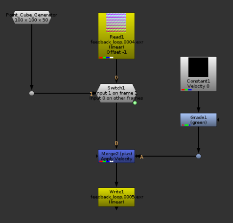
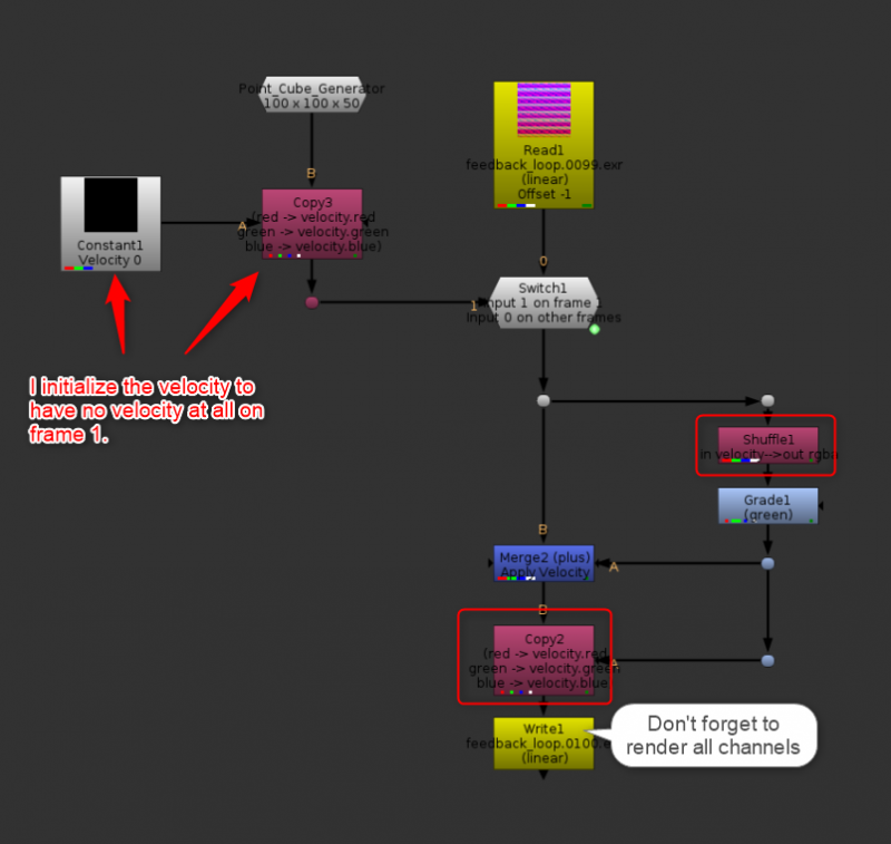
We now have a branch where our velocity is calculated, it’s then simply applied with a plus.
Let’s add Inertia
So far, our Velocity branch brings us very little value. This is due to the fact that it is disconnected from our feedback loop. In the setup above, we always initialized the Velocity to be zero, and re-calculated from scratch. What would happen if instead we were to use the velocity from the previous frame as the starting point for our new velocity vector?
The falling cube, now with velocity channel.
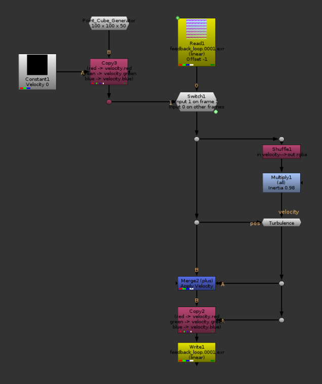
I had to reduce the downward force quite a lot, otherwise the cube was out of frame in just a couple of frames. Notice how the cube’s speed is now exponential (alright, I admit it’s hard to tell, but look at the speed at the beginning VS the speed at the end). This is because of inertia. On each frame, we start with a velocity vector that is already the speed of the previous frame, and we re-apply the downward force on top of it. It is starting to look a bit more physical doesn’t it.
Let’s try the same thing, but with increased gravity (Grade1) and add an initial velocity up (Constant1) of 0.25. I’m also going to push the camera a bit further so we can see more of the movement happening.
The cube, now with an initial velocity upwards, slowing down because of gravity before falling back down. It’s starting to look more interesting.
There isn’t enough Friction between us
The example above is semi physical. I wouldn’t really call any of this physical between I’m not basing any of the math on reality. The example above of the cube moving up and falling back down would sort of match what would happen on Earth in a Vacuum. We’re missing an important element, and that element is Air. More specifically Air Friction.
Simulating proper air displacement and friction is way past my knowledge at this point, but there is a way to cheat it, and most particle systems actually do use that same cheat: Drag.
While we could implement a physically correct version of drag, the most common and simple way to do it is to say: In each frame, air resistance is killing 5% of my inertia. This is easy because all we need is a multiply node. To reduce the inertia by 5%, we just multiply by 0.95. For 10%: 0.9, 50%: 0.5, you get it.
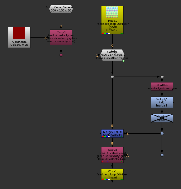
Don’t need gravity for this example, and I replaced the initial velocity by 0.25 in x instead of y. The Multiply node is my Drag (but it’s working backwards, higher values represent less Drag, lower values more drag)
Different values of Drag. You don’t need much drag to slow down the cube quite a lot. Even a 10% drag brings it almost to a total stop rather quickly (in theory, it would never reach exactly 0 velocity, but since math precision is limited, it actually happens rather fast.
Attraction and Repulsion
We have the basics laid down, but let’s start adding a bit more fun. I would like to create point (or radial) forces. How would we do that? Well it turns out that if we subtract the position of our points from the position of our point force, the resulting vector applied as a velocity would instantaneously bring all the points to our point force position.
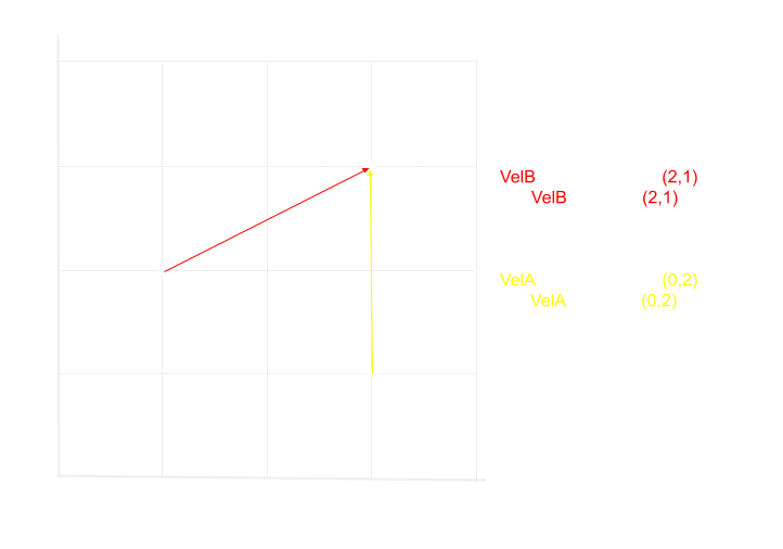
Example of subtracting vectors, in 2D.
Now of course this is not really what we are aiming for exactly, we do not want the whole cube to collapse into 1 point instantaneously. Even if we were to divide the velocity by 10, it would still collapse into a single frame in 10 frames instead of one. If you try it yourself, or draw it on paper, you will notice that the points that are the furthest away from the point force are getting the strongest forces, and the closer ones are getting less affected. This is the opposite of what I want here. I would like the points closest to my force to be the most affected, and have my force decrease intensity as I get away from it.
We can try to normalize the force vectors, if you remember the basics of vectors, they have a direction and a magnitude. By normalizing them, we keep the direction, but we force the magnitude to be 1. This can create some interesting results. I thought this step would be necessary when I started experimenting with the radial forces, and while I like some of the results it created, I found out later that it doesn’t really achieve what a magnet for example would do.
All w need to do is multiply the magnitude by any value that we want. I can use a PMatte as my Multiplier which pretty much achieves what I am aiming for.
With Repulsion.
With Attraction.
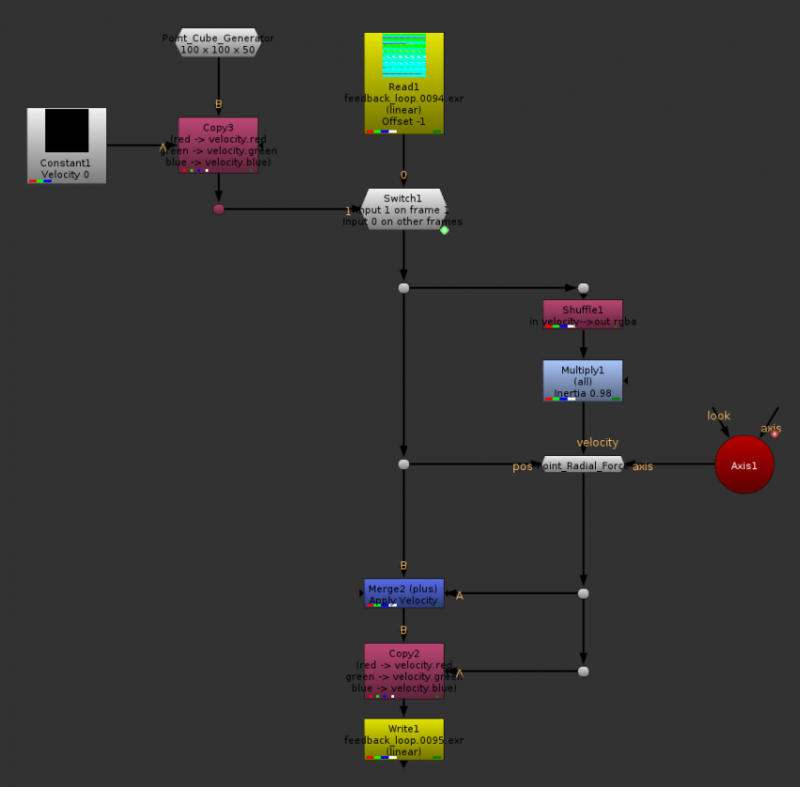
Setup with the Radial Force. I’ll include the node in the .nk scene that you can download at the bottom of this article.
At this point, as you can notice, we’ve got something that is pretty close to a traditional particle system. We actually had it when we introduced inertia, but we didn’t really have any interesting forces at that time. Let’s create a few more forces before wrapping up.
Turbulence
A cool force we often find in particle systems, is some sort of turbulence, which sends your particle swirling in the air. This is a bit what the fractal evolve from Higx does, but let’s do our own.
The basic idea is simple, you can use an expresion node with the fBm() function, feeding in the position as x, y and z arguments, and that would give you what is frequently called a PNoise. A Noise based on a 3D coordinate. Actually, even the default noise in Nuke uses that, giving you the equivalent of the noise on a 3D card. As we need to obtain 3 colors to define a random 3d vector, we can repeat the operation above 2 more times, offsetting some values. For example, for the second one you could use z+100, and for the third, z+200.
In my case, I wanted to do things a bit fancier, so I used a blinkscript to generate the noise. Funnily enough, I used my 4D noise kernel as a base (from spin_nuke_gizmos’s Noise3d), which itself was using some code from 4D_Noise made by Mads, which is also the base for the fractal nodes included in Higx.
Without going into full details, the advantage of 4d noise is that the 4th dimension can be used to “evolve” the noise without seeing it slide in a particular axis. In that case I use the 4th dimension as a different seed for my x, y and z axis.
A relatively large amplitude, low_frequency turbulence.
Masking
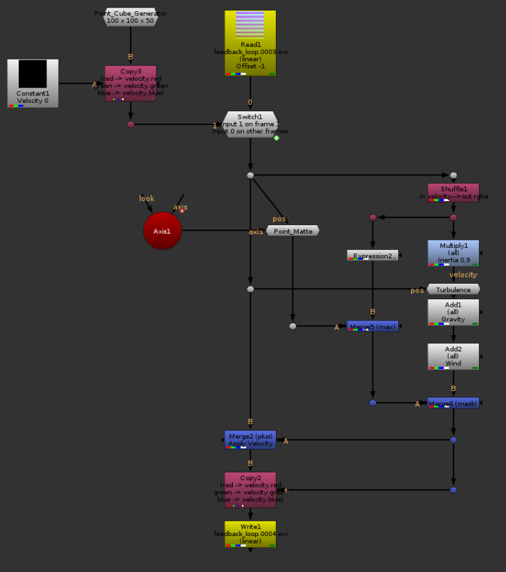
Just like you can use any sort of 2D or P masking with the default tools in Higx, we can do the same here, but one of the new advantages is that we can use them to define which force will affect which point. For example, I will use a P_Matte to define which points are going to be affected by motion, so that by default my points aren’t moving, but will only start moving when in contact with the P_Matte. Once in motion, a point should keep being affected by forces.
Wind, turbulence, gravity, masked.
Ground Plane and Collisions
Wouldn’t it be neat if we could get our points to hit some geometry and stop, or bounce? While doing it with a custom geometry is a bit hard with the default nodes from Nuke, doing a ground plane is a very simple thing. The easiest version of a ground plane would be to clamp the negative values in your Y channel. No point can now be under the ground floor, done.
That is a bit too simple, so let’s get some bounce, shall we?

When a vector crosses the ground plane, we want to find out the portion of it that is under the ground plane, and bounce it back in Y.
In order to do this, I will replace the merge node (Merge2) that we have been using so far to apply the velocity with a custom node. There I will first check if applying the vector would bring the point under 0 in Y. If it would, I will split the vector into two parts, the part that would bring the point in contact with the ground, and the part that would bring it underground. There, I can flip the Y of the second vector, and multiply it with a value of my choice that would represent how bouncy the floor it. Finally, I need to set the new velocity in the direction of the bounce, so that inertia would keep it going.
The same setup as above, but with a ground plane and some bounce. This is the .nk I will be sharing.
Just gravity and bounce, to show the bounce a bit more obviously.
These examples aren’t particularly pretty, but I’m leaving this to you.
Conclusion
We have seen a few different forces we could apply to our particle system, and the possibilities are already starting to be good, but remember how we have seen at the beginning of this article that nuke’s particle system had 11 channels of properties that could be used to simulate the particles? Well so far we’ve only used 2, but nothing stops us from adding more! We have no limits here, except for Nuke’s 1024 channels limit. You could add a mass channel, and have the heavier points being less affected by the drag than the light points. You could have a temperature channel, with a warm point force which can be used as a multiplier on the motion, so that a cold point cannot move, but starts moving as it warms up and melts. You could add any arbitrary parameter that you could think of really. I’m not going to do that for you, but the whole point of this article was to show you that yes, you’re probably able to develop your own custom particle system.
Get the script here.


Hey Hi!
First of all, really great article!! I’m trying to rebuild some examples and i downloaded the script you’ve provided,
but i can’t figure out wich one of the nodes the RadialForce is….any help? 🙂
It is the one named Point_Radial_Force, not connected to the rest of the tree on the right side.
Hey Erwan. indeed as the first comment makes note.. first off, thanks for so many great contributions throughout the Nuke community over the years.
Second, quick Nuke particle question.. in the paragraph of this article ‘Ground Plane and Collisions’, “Wouldn’t it be neat if we could get our points to hit some geometry and stop, or bounce? While doing it with a custom geometry is a bit hard with the default nodes from Nuke”
Do you mean it’s possible? I’ve made a sim of some ambient dust particles in Nuke and I’m trying to use ParticleBounce with the bounce and drag set to 0. External bounce on. Along with some custom geo I made as a collider to represent a figure running through the shot. Once plugged in, the particles disappear from the scanline render.
Many thanks again!
Here this was an experiment at making a particle system without using the built-in particle system. The particle bounce node should do what you need, but I found it a bit hard to set up, and it has a tendency to break things. The 2 most common ways to make a collider are to either convert the geometry to an SDF and use the distance field to calculate whether the particles are inside or outside the volume, or to do intersection tests on the polygons in the path of the particle.
I am not sure which one nuke uses, but from not seeing any other volumetric type of nodes, I’m assuming it’s doing the second method. That would mean that for each particle in your scene, Nuke needs to check whether it hit any polygon in your scene. It’s an exponential calculation. For 1 particle and 1 polygon, you get 1 check. 2 particles 2 polygons you get 4, etc… I’d keep your collider as simple as possible and number of particles low, until you get to a point where things are working, then increase the particle count in steps. If it breaks again, reduce the number a bit. Also make sure your collider has normals.