
For the very few of you who have missed it, the talented Mads Hagbarth recently released his Higx PointRender.
While the tool is not free, it’s pretty affordable compared to what some others might charge for tools that can accomplish this much.
There are a few video tutorials on the official website, plus some experiments on Xavier Martin’s blog, but that is more or less the extent of it for now.
I am not going to produce anything as pretty as what Xavier made, but I thought it could help a few to have access to a couple more experiments, and I will try to explain a little bit what the tool is and how it works, so that you are armed to push it further.
One thing that always struck me about Mads’ tools is that it’s always both simple and genius at once. When I check out one of his new tools I always get extremely impressed, and once I look at how it’s achieve I always feel dumb for not having thought about it before.
Higx is open-source, meaning that when you buy the tool, you have access to all the code and all the gizmos are open for you to break down.
Mads is selling it on a trust basis, and as a result I will not be able to include real nuke snippets including his nodes, as that would be as if I was redistributing the nodes themselves for free.
What is it? Is it a particle system?
Point_Render is not a particle system, not really. Let’s focus on the PointRender Node itself for a bit.
The PointRender node, to its core, is extremely simple. It uses two layers: rgba and pos. For each pixel in the image, it will define a 3D position based on the pos channels. It will then calculate where on the 2D plane this point would be if shot through the attached camera, and draw a pixel of the color from rgba at that 2d position.
As the name says, it is only a render engine, to the same extent that the ScanlineRender node is only a render engine.
The beauty of it, is that it doesn’t use the 3D workspace of Nuke, which can be a bit slow, but instead uses 2D image data to represent all the 3D data. If we imagine a single pixel, with RGB values of 0, 1, 0 and pos values of 1, 1, 1, that would correspond to a green point, at coordinate x=1, y=1, z=1.
If that reminds you of something, it should, as that is the same logic used for position passes when rendering CG (or any other AOV, though the other passes are storing different data into pixels).
The great thing about all this, is that we can use regular 2D nodes to manipulate all that data and get really awesome results. The amount of flexibility is huge. That also means tools like P_Mattes or P_Noises would work perfectly on Points data.
The other nodes included with PointRender are utilities that would help you to get some cool results from it. Some of them sort of pretend that our data is like a traditional particle engine and do make it look like a particle simulation, but there actually isn’t any simulation involved here, which makes it really fast, but also less advanced than regular particles out of the box. With traditional particles, one of the important points is that the position of a particle at any given frame depends on its position at previous frames. With PointRender, every frame is pretty much independent from the others.
How do we get started?
To really make sure we understand how the tool works, we’re going to start without involving the tool at all (and this way I’ll be able to share the setup with you).
We’ll start really boring, trying to make a point cloud representing a checkerboard on a card.
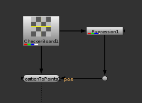
Simple setup. I made the Checkerboard 256×256 for speed.
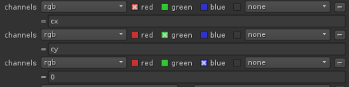
The default expression cx and cy does a great job here at giving us x and y coordinates, and we just set z manually.
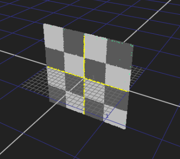
Result in 3D Viewer
set cut_paste_input [stack 0]
version 11.2 v4
CheckerBoard2 {
 inputs 0
 format "256 256 0 0 256 256 1 square_256"
 name CheckerBoard1
 selected true
 xpos -19
 ypos -140
}
set Nd673f10 [stack 0]
Expression {
 expr0 cx
 expr1 cy
 expr2 0
 name Expression1
 selected true
 xpos 151
 ypos -116
}
Dot {
 name Dot1
 tile_color 0xcccccc00
 selected true
 xpos 185
 ypos -29
}
push $Nd673f10
PositionToPoints2 {
 inputs 2
 display textured
 render_mode textured
 name PositionToPoints1
 selected true
 xpos -19
 ypos -32
}
Now, if you’re unsure at this stage how the RGB value coming from the expression node controls the 3D point position, I invite you to play with this a bit. Drop a grade node between the expression and the PositionToPoints and observe how you can scale things up and down with gain and multiply, or how you can move things in 3D space playing with offset. See what happens if you clamp negatives or not, etc..
At this point, our point cloud is fairly boring. Let’s add some noise in the blue channel and see what happens.
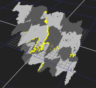
That is starting to be more interesting, let’s render this with a ScanlineRender and a Camera. Let’s also tweak the PositionToPoints node to make the point size 1 and point details 1 as well.

Point cloud rendered via the ScanlineRender
It doesn’t look too bad, but let’s setup the same render via PointRender now. In order for PointRender to understand our data, we have to copy our position data into a layer called ‘pos’. You can do that through a Copy or a ShuffleCopy for example.
Here is my setup, as well as the render from the PointRender node:
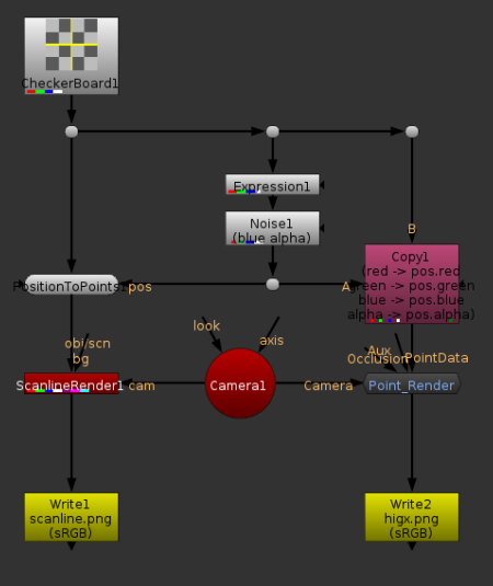
Setup showing both the ScanlineRender Setup and the Higx render.
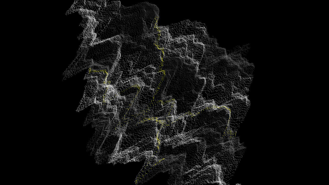
Rendered with higx PointRender.
With this amount of point, there isn’t really a clear winner. Both renders look slightly interesting, but neither is stunning. The ScanlineRender rendered bigger points, but other than that you can’t really tell.
Remember how I said earlier that one pixel = 1 point. In this case I was using a 256×256 checkerboard as a source, which gave me roughly 65K points. Let’s try increasing the number of points. Doubling the image resolution to 512*512 would give me ~260K, Four times as many as my previous render. In order to preserve the appearance of my noisy checkerboard, I’m going to change that resolution via a reformat, in impulse on my RGB, and in cubic on position data. I do it this way because increasing the resolution of the reformat directly would affect the number of checkers on the checkerboard, and the noise scale would be different. I’m actually going to go directly to 1024*1024, for a cool million points.
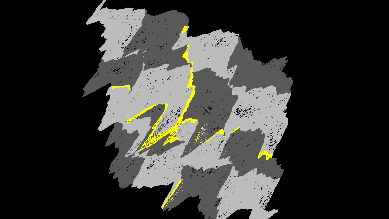
A million points rendered with the ScanlineRender
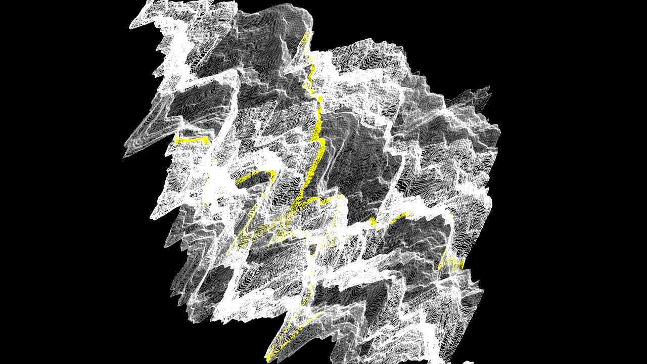
A million points rendered with the PointRender
Now the difference is starting to show. On my side, one of the differences was how long it took to render. PointRender barely felt the hit of going to a million points, while PositionToPoints+ScanlineRender had to think about it for a bit. On the results side, you can notice how the scanline render has all the points respect exactly the color coming in from the RGB input. Each square of the checkerboard keeps its flat color from the input. In PointRender, you can see that it looks brighter in some areas than others. This is because it renders the points in an additive mode. If two points overlap each other, the pixel will be the result of point A + point B. If there are 3 points it will get even brighter, etc.. That is a bit closer to how we perceive light or plasma (don’t know if that is physically correct, but in perception at least).
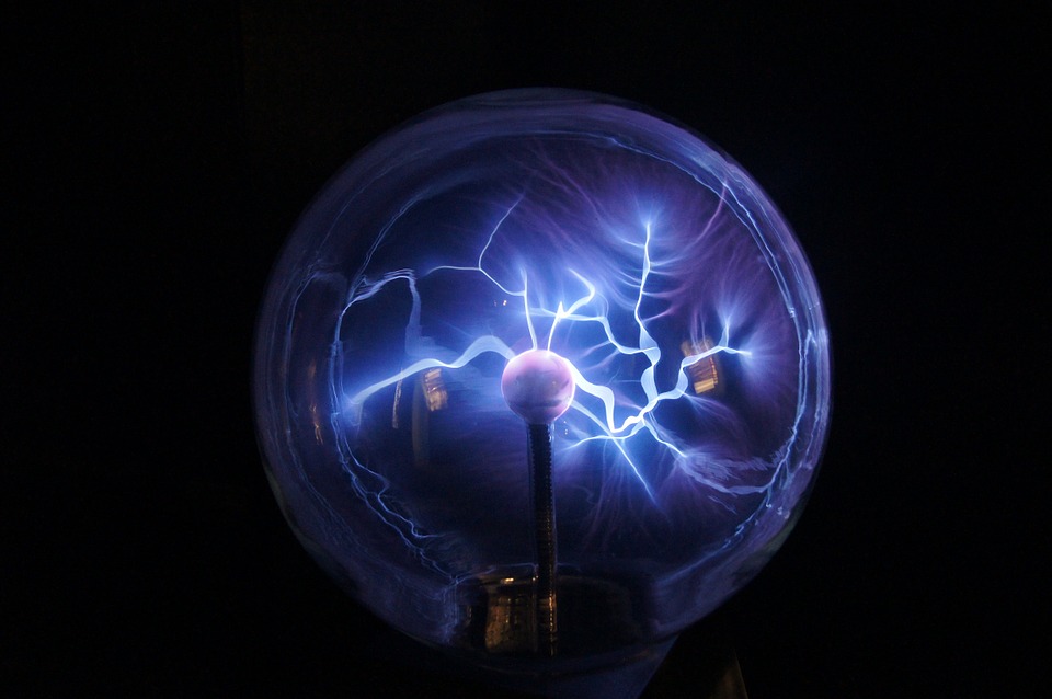
Photo of a plasma ball
With even more points, reduced exposure, and a bit of color correction and glow, we can get pretty close to look like the photo above (in terms of look, not shape).
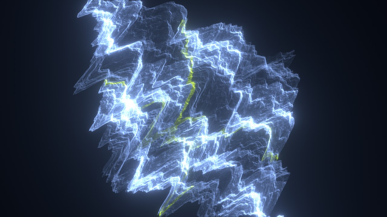
Render with 4 million points, graded and glowed
The other Higx nodes
We’re starting to be able to get something kind of cool looking, yet we haven’t even used any of the other higx tools aside from the point render.
They come in 4 categories: General, Generator, Modifier, Shader
- General: This is where the PointRender node lives, along with a Point3D_Preview node, which is actually just a PositionToPoint that has been preset to use the passes as PointRender does.
- Generator: These are the starting points. In our test above, we used an expression node to set the initial world position. These generators can be used to generate different primitives (sphere, torus, cylinder, …) or generate points from a geometry. The Geometry source is limited to a million points, but if you have UVs on the geometry you can render the position pass in UV mode from a scanline render at high res to get more points.
- Modifier: These tools allow you to move points around. The fractal and fractal evolve add a sort of turbulence on the points, much like we did with the Noise above (would be very similar to the fractal node if we stared to animate our noise). The fractal evolve is doing the same, but in a recursive manner, which makes the particle seem like they get further and further from their starting point, and making it look like a particle simulation. It’s pretty awesome actually.
- Shader: These nodes generate colors based on the position data. Some can do some sort of relighting, calculate velocity, etc..
I’m not really going to cover any of these nodes because they are fairly easy to grasp and use, and because they are the nodes used in most other tutorials. I’m more interested in doing a few experiments and see what we can do with the PointRender.
Making a 3D scope
We have cool scopes in Nuke, but how about we try to make our own so that we can render it out and use it for some cool motion-graphicky elements. For the sake of using a familiar image, I’m going to dig up good old Marcie.

Marcie
Marcie, as viewed through the eyes of our scopes
Marcie 3D
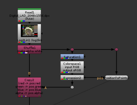
Setup for Marcie 3D. It’s basically the same setup as our previous experiment, except this time I use the luma of the image in the Z channel instead of a noise. I converted the luma to sRGB so that it would be less spiky but you don’t need to.
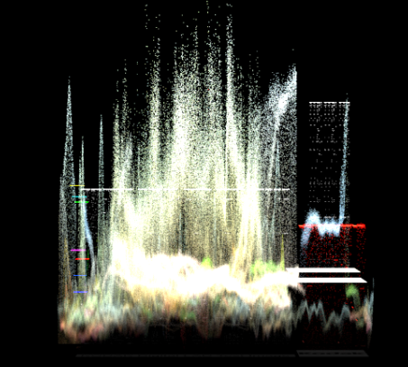
3d Marcie rendered with PointRender from a camera at the bottom facing up.
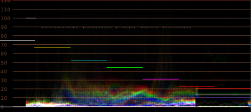
PointRender doesn’t seem to support every type of camera at the moment. Ideally I would have rendered this with an orthographic camera. Since higx is open-source, we could go in and change the way it calculates the camera matrix, but that is a bit beyond the scope (pun intended?) of this article. Some other scopes rendered with PointRender, and their setup under.
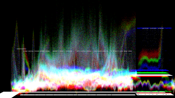
Closer to a proper waveform. We could easily kill the perspective by making the Y channel 0, making it a flat point cloud.
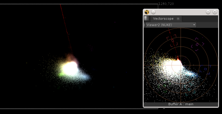
Another scope, a VectorScope, with a comparison to an actual VectorScope from Nuke.
set cut_paste_input [stack 0]
version 11.2 v4
BackdropNode {
 inputs 0
 name BackdropNode1
 tile_color 0x667f71ff
 label Luma
 note_font_size 40
 selected true
 xpos 1085
 ypos -214
 bdwidth 330
 bdheight 293
}
BackdropNode {
 inputs 0
 name Backdrop_VectorScope
 tile_color 0x667f6aff
 label Waveform
 note_font_size 40
 selected true
 xpos 1474
 ypos -244
 bdwidth 427
 bdheight 378
}
BackdropNode {
 inputs 0
 name Backdrop_Vectorscope
 tile_color 0x6c7f66ff
 label Vectorscope
 note_font_size 40
 selected true
 xpos 1970
 ypos -244
 bdwidth 325
 bdheight 337
}
push $cut_paste_input
Dot {
 name Dot8
 tile_color 0xcccccc00
 label Image
 selected true
 xpos 1169
 ypos -329
}
Shuffle {
 alpha white
 name Shuffle1
 label "make alpha white"
 selected true
 xpos 1135
 ypos -275
}
Dot {
 name Dot6
 tile_color 0x9e3c6300
 selected true
 xpos 1169
 ypos -144
}
set N258c9320 [stack 0]
Saturation {
 saturation 0
 name Saturation1
 selected true
 xpos 1135
 ypos -93
}
Colorspace {
 colorspace_out sRGB
 name Colorspace1
 label "input \[value colorspace_in]\noutput \[value colorspace_out]"
 selected true
 xpos 1135
 ypos -70
}
Expression {
 expr0 cx
 expr1 cy
 name Expression2
 selected true
 xpos 1135
 ypos -22
}
Dot {
 name Dot5
 tile_color 0xcccccc00
 selected true
 xpos 1169
 ypos 14
}
push $N258c9320
Dot {
 name Dot7
 tile_color 0x9e3c6300
 selected true
 xpos 1319
 ypos -144
}
set N25897250 [stack 0]
PositionToPoints2 {
 inputs 2
 display textured
 render_mode textured
 name PositionToPoints2
 selected true
 xpos 1285
 ypos 11
}
push $N25897250
Dot {
 name Dot9
 tile_color 0x9e3c6300
 selected true
 xpos 1660
 ypos -144
}
set N1217dfc0 [stack 0]
Colorspace {
 colorspace_out sRGB
 name Colorspace2
 label "input \[value colorspace_in]\noutput \[value colorspace_out]"
 selected true
 xpos 1626
 ypos -104
}
set Nc2fb4f0 [stack 0]
Shuffle {
 red black
 green black
 alpha white
 name Shuffle4
 label "in \[value in]-->out \[value out]"
 selected true
 xpos 1720
 ypos -56
}
Expression {
 expr0 cx
 expr1 cy
 expr2 r+g+b
 name Expression5
 selected true
 xpos 1720
 ypos -20
}
push $Nc2fb4f0
Shuffle {
 red black
 blue black
 alpha white
 name Shuffle3
 label "in \[value in]-->out \[value out]"
 selected true
 xpos 1626
 ypos -56
}
Expression {
 expr0 cx
 expr1 cy
 expr2 r+g+b
 name Expression4
 selected true
 xpos 1626
 ypos -20
}
push $Nc2fb4f0
Shuffle {
 green black
 blue black
 alpha white
 name Shuffle2
 label "in \[value in]-->out \[value out]"
 selected true
 xpos 1524
 ypos -59
}
Expression {
 expr0 cx
 expr1 cy
 expr2 r+g+b
 name Expression3
 selected true
 xpos 1524
 ypos -16
}
ContactSheet {
 inputs 3
 width 2048
 height 4668
 columns 1
 name ContactSheet1
 selected true
 xpos 1626
 ypos 17
}
set N26db1d90 [stack 0]
Grade {
 white {2 1 1 1}
 white_panelDropped true
 black_clamp false
 name Grade2
 selected true
 xpos 1625
 ypos 41
}
Dot {
 name Dot10
 tile_color 0x7aa9ff00
 selected true
 xpos 1661
 ypos 69
}
push $N26db1d90
Expression {
 expr0 y>=height/3*2
 expr1 "y<height/3*2 && y>=height/3"
 expr2 y<height/3 name Expression6 selected true xpos 1771 ypos 17 } PositionToPoints2 { inputs 2 display textured render_mode textured name PositionToPoints3 selected true xpos 1771 ypos 66 } push $N1217dfc0 Dot { name Dot11 tile_color 0x9e3c6300 selected true xpos 2054 ypos -144 } set Nbbee630 [stack 0] Dot { name Dot12 tile_color 0x9e3c6300 selected true xpos 2199 ypos -144 } Colorspace { colorspace_out YCbCr name Colorspace3 label "input \[value colorspace_in]\noutput \[value colorspace_out]" selected true xpos 2165 ypos -85 } Shuffle { red green green red name Shuffle5 label "in \[value in]-->out \[value out]"
 selected true
 xpos 2165
 ypos -37
}
Grade {
 white {1 0 1 1}
 white_panelDropped true
 black_clamp false
 name Grade3
 selected true
 xpos 2165
 ypos 25
}
push $Nbbee630
PositionToPoints2 {
 inputs 2
 display textured
 render_mode textured
 name PositionToPoints4
 selected true
 xpos 2020
 ypos 25
}
Making Dust in a volume ray
As I mentioned, the position pass used for PointRender is the same as what we’ve been working with for things like PWorld passes, and as a result all the P tools can be used on it. They could also be considered vectors, and as a result the whole range of vector tools such as the ones I have published before could be used as well. Now, these are starting to date a little. Mathieu Goulet-Aubin and myself have been working on a new collection of such tools, which can be found on github here. It’s not quite finished yet, but these are great weapons to manipulate this 3D data.
Now, making scopes was cool, but it’s not something we need every day. Adding some dust in a god ray is a bit more frequent. Clients just love these godrays, and we usually have to rely on particles to do that.
Let’s start by defining the scope of the work. We’ll need a sort of volume container with a bunch of dust inside, we’ll need to make that dust move, and we’ll need to light it as if rays were coming through. For the generator, we’ll have to come up with a custom one, as there isn’t really a volume generator included. To make the dust move, Point_Fractal will be perfect, so that is done. For the lighting as if a godray was present, there is no such thing included, but some existing Nukepedia tools can help there.
How would we generate a volume (cube, to be simple) with a bunch of random points inside? One relatively easy solution would be to use noise, with a tiny little size. This way, each pixel would have a seemingly random value between 0 and 1. Do 3 such noises with slightly different values and shuffle in r, g and b, and you’ve got a cube full of random points. However, due to the nature of the noise tool, I’m going to make a custom expression node in this case.
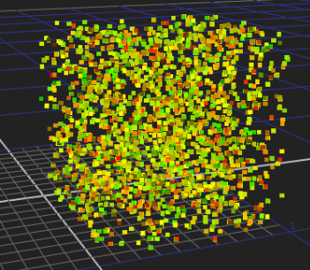
Cube filled out with random points
set cut_paste_input [stack 0]
version 11.2 v4
push $cut_paste_input
Expression {
expr0 "random(x_seed, x*20, y)"
expr1 "random(y_seed, x*50, y*10)"
expr2 "random(z_seed, x*10, y*100)"
expr3 "random(a_seed, x, y)"
name Expression7
selected true
xpos 2896
ypos -158
addUserKnob {20 User}
addUserKnob {3 x_seed}
x_seed 20
addUserKnob {3 y_seed}
y_seed 40
addUserKnob {3 z_seed}
z_seed 60
addUserKnob {3 a_seed}
a_seed 80
}
We now have our little 1×1 cube. Most likely the scene is larger than that so you can use Higx’s built in Point_Transform to place the points where they are needed in the scene.
You can also add the Point_Fractal, to make the points move around. As always, changing the resolution of the image would change the number of points. Okay, so that was surprisingly easy, we’ve got randomly moving random points already. How do we make the light ray now?
I can use a tool such as Reproject_3D from the Spin Nuke Gizmos (itself an adaptation of ReProject3D). I prefer to use the Spin version as it’s a little bit more user friendly in my opinion. So all I need to do is setup a projection camera, and project some texture through my point cloud.
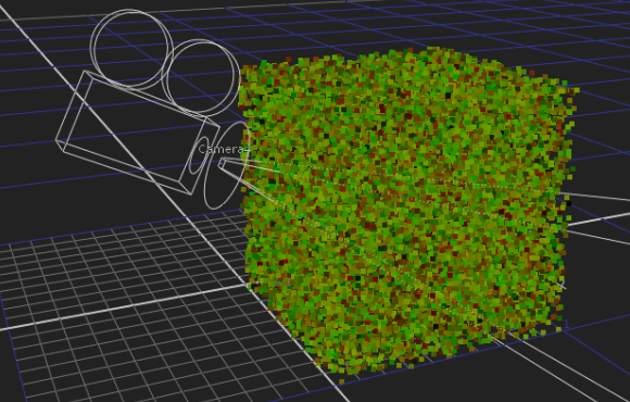
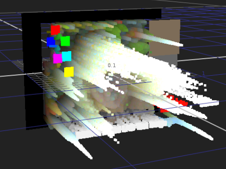
Adding a projection camera
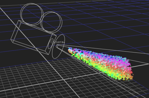
Projecting a ColorWheel through the point cloud.
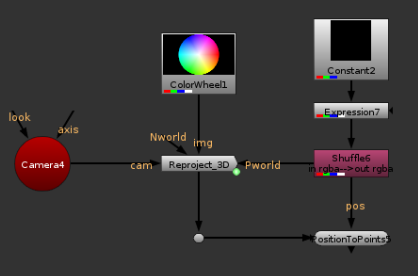
The setup for the image above
Now instead of projecting just a color wheel, let’s make a texture that would be a bit more reminiscent of a light ray. I’m also going to use a good old P_Matte to gain down the dust that is further away from the camera.
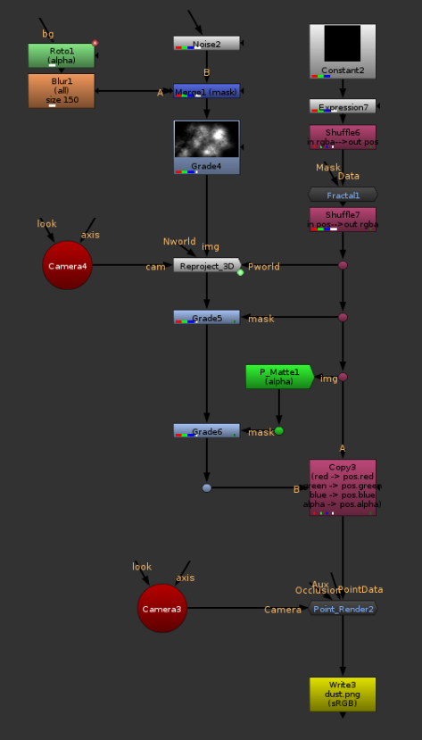
A slightly more complete setup, using some higx nodes.
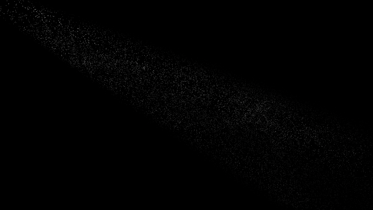
Resulting dust ray. It’s a bit boring as a still, but it’s actually pretty sweet in motion.
Going Further
This post is starting to be a bit lengthy, but we’ve only really only scratched the surface. I could keep going on for a while, but instead I will be splitting the next subject I wanted to cover into another article. There, we’ll be pushing PointRender further than what it was intended for, and see how we could make it do actual particle simulation, with forces (gravity, magnets, wind, etc..) and even simple collisions (ground plane). Stay posted.
This is an awesome introduction and well explained article. Thank you for sharing! Looking forward to reading your next one.
Thanks Erwan! Really like your vector tools. But when I tried to install the new vector set you and Mathieu made, the init.py file (which recursively add subfolders to the plugin path) cannot be interpreted by nuke. An error will occur and Nuke won’t open up. Could you help? Thanks!
Yes, these tools aren’t quite done.
It’s most likely because I used scandir which isn’t installed by default. You can replace scandir with os.walk in the init.py and menu.py and it should work. I’ll be doing that soon.
Hi Lisa, the Vector Tools menu has been fixed since.
Great introduction, thank you very much Erwan.
Thank you so much for the explanation and breakdown!